ML | Linear Regression using Python.

Meaning of Regression
Regression attempts to predict one dependent variable (usually denoted by Y) and a series of other changing variables (known as independent variables, usually denoted by X).
Linear Regression
Linear Regression is a way of predicting a response Y on the basis of a single predictor variable X. It is assumed that there is approximately a linear relationship between X and Y. Mathematically, we can represent this relationship as:
Y ≈ ɒ + ß X + ℇ
where ɒ and ß are two unknown constants that represent intercept and slope terms in the linear model and ℇ is the error in the estimation.
Example
Let’s take the simplest possible example. Calculate the regression with only two data points.

Here we have 2 data points represented by two black points. All we are trying to do when we calculate our regression line is draw a line that is as close to every point as possible.

Here, we have a perfectly fitted line because we only have two points.Now, we have to consider a case where there are more than 2 data points.

By applying linear regression we can take multiple X’s and predict the corresponding Y values. This is depicted in the plot below:

Our goal with linear regression is to minimise the vertical distance between all the data points and our line.
So now I guess, you have got a basic idea what Linear Regression aims to achieve.
Before Applying any machine algorithm do Data Preparation Process to get the better results
Data Preparation Process
The more disciplined you are in your handling of data, the more consistent and better results you are like likely to achieve. The process for getting data ready for a machine learning algorithm can be summarized in three steps:
- Step 1: Select Data
- Step 2: Preprocess Data
- Step 3: Transform Data
Step 1: Select Data
This step is concerned with selecting the subset of all available data that you will be working with. There is always a strong desire for including all data that is available, that the maxim “more is better” will hold. This may or may not be true.
You need to consider what data you actually need to address the question or problem you are working on. Make some assumptions about the data you require and be careful to record those assumptions so that you can test them later if needed.
Below are some questions to help you think through this process:
- What is the extent of the data you have available? For example through time, database tables, connected systems. Ensure you have a clear picture of everything that you can use.
- What data is not available that you wish you had available? For example data that is not recorded or cannot be recorded. You may be able to derive or simulate this data.
- What data don’t you need to address the problem? Excluding data is almost always easier than including data. Note down which data you excluded and why.
It is only in small problems, like competition or toy datasets where the data has already been selected for you.
Step 2: Preprocess Data
After you have selected the data, you need to consider how you are going to use the data. This preprocessing step is about getting the selected data into a form that you can work.
Three common data preprocessing steps are formatting, cleaning and sampling:
- Formatting: The data you have selected may not be in a format that is suitable for you to work with. The data may be in a relational database and you would like it in a flat file, or the data may be in a proprietary file format and you would like it in a relational database or a text file.
- Cleaning: Cleaning data is the removal or fixing of missing data. There may be data instances that are incomplete and do not carry the data you believe you need to address the problem. These instances may need to be removed. Additionally, there may be sensitive information in some of the attributes and these attributes may need to be anonymized or removed from the data entirely.
- Sampling: There may be far more selected data available than you need to work with. More data can result in much longer running times for algorithms and larger computational and memory requirements. You can take a smaller representative sample of the selected data that may be much faster for exploring and prototyping solutions before considering the whole dataset.
It is very likely that the machine learning tools you use on the data will influence the preprocessing you will be required to perform. You will likely revisit this step.
Step 3: Transform Data
The final step is to transform the process data. The specific algorithm you are working with and the knowledge of the problem domain will influence this step and you will very likely have to revisit different transformations of your preprocessed data as you work on your problem.
Three common data transformations are scaling, attribute decompositions and attribute aggregations. This step is also referred to as feature engineering.
- Scaling: The preprocessed data may contain attributes with a mixtures of scales for various quantities such as dollars, kilograms and sales volume. Many machine learning methods like data attributes to have the same scale such as between 0 and 1 for the smallest and largest value for a given feature. Consider any feature scaling you may need to perform.
- Decomposition: There may be features that represent a complex concept that may be more useful to a machine learning method when split into the constituent parts. An example is a date that may have day and time components that in turn could be split out further. Perhaps only the hour of day is relevant to the problem being solved. consider what feature decompositions you can perform.
- Aggregation: There may be features that can be aggregated into a single feature that would be more meaningful to the problem you are trying to solve. For example, there may be a data instances for each time a customer logged into a system that could be aggregated into a count for the number of logins allowing the additional instances to be discarded. Consider what type of feature aggregations could perform.
You can spend a lot of time engineering features from your data and it can be very beneficial to the performance of an algorithm. Start small and build on the skills you learn.
Steps for Linear Regression:
1. Importing the necessary Libraries & dataset.
2. Splitting the dataset into the Training set and Test set.
3. Fitting Simple Linear Regression to the Training set.
4. Predicting the Test set results.
5. Scatter plot of y_test vs Prediction.
6. Distplot...( Should come Normal distribution otherwise eliminate Linear Reg )
7. Visualizing the Training set results ( Optional )
8. Visualizing the Test set results ( Optional )
9. Lets Predict...!
10. Also Calculate: coef_ , intercept_ , MAE , MSE , RMSE , r2_score.
Code for Linear Regression:
In the below code snippet I have assumed the dataset is stored in the variable df.

To find Accuracy, Mean Absolute Error, Mean Squared Error, Root Mean Squared error execute the following code.
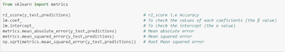
Please also import this in below code since i have forget to mention sklearn.metrics import r2_score.

Mathematical Formula for all the above error

No comments:
Post a Comment