Logistic regression is the most famous machine learningalgorithm after linear regression. In a lot of ways, linear regression and logistic regression are similar. But, the biggest difference lies in what they are used for. Linear regression algorithms are used to predict/forecast values but logistic regression is used for classification tasks.
There are many classification tasks done routinely by people. For example, classifying whether an email is a spam or not, classifying whether a tumour is malignant or benign, classifying whether a website is fraudulent or not, etc. These are typical examples where machine learning algorithms can make our lives a lot easier. A really simple, rudimental and useful algorithm for classification is the logistic regression algorithm. Now, let’s take a deeper look into logistic regression.
Sigmoid Function (Logistic Function)
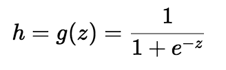
Logistic regression algorithm also uses a linear equation with independent predictors to predict a value. The predicted value can be anywhere between negative infinity to positive infinity. We need the output of the algorithm to be class variable, i.e 0-no, 1-yes. Therefore, we are squashing the output of the linear equation into a range of [0,1]. To squash the predicted value between 0 and 1, we use the sigmoid function.
Squashed output-h
We take the output(z) of the linear equation and give to the function g(x) which returns a squashed value h, the value h will lie in the range of 0 to 1. To understand how sigmoid function squashes the values within the range, let’s visualize the graph of the sigmoid function.
As you can see from the graph, the sigmoid function becomes asymptote to y=1 for positive values of x and becomes asymptote to y=0 for negative
Cost Function
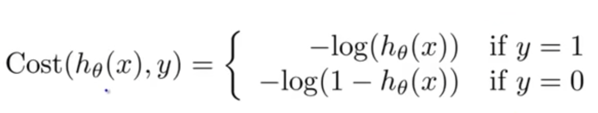
Since we are trying to predict class values, we cannot use the same cost function used in linear regression algorithm. Therefore, we use a logarithmic loss function to calculate the cost for misclassifying.
The above cost function can be rewritten as below since calculating gradients from the above equation is difficult.
Here h teta (x) is our predictions.
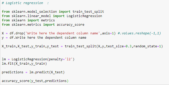
Code
In above code i have assumed that the data is stored in the variable df
Conclusion
Logistic regression is a simple algorithm that can be used for binary/multivariate classification tasks. I think by now you would’ve obtained a basic understanding of how logistic regression algorithm works. Hope this article was helpful :)
Random Forests algorithm has always fascinated me. I like how this algorithm can be easily explained to anyone without much hassle. One quick example, I use very frequently to explain the working of random forests is the way a company has multiple rounds of interview to hire a candidate. Let me elaborate.
Say, you appeared for the position of a Statistical Analyst at WalmartLabs. Now like most of the companies, you don’t just have one round of interview. You have multiple rounds of interviews. Each one of these interviews is chaired by independent panels. Each panel assesses the candidate separately and independently. Generally, even the questions asked in these interviews differ from each other. Randomness is important here.
The other thing of utmost importance is diversity. The reason we have a panel of interviews is that we assume a committee of people generally takes better decision than a single individual. Now, this committee is not any collection of people. We make sure that the interview panel is a little diversified in terms of topics to be covered in each interview, the type of questions asked, and many other details. You don’t go about asking the same question in each round of interviews.
After having all the rounds of interviews, the final call whether to select or reject the candidate is based on the majority of the decision from each panel. If out of 5 panel of interviewers, 3 recommends a hire and two against a hire, we tend to go ahead with selecting the candidate. I hope you get the gist.
If you have heard about the decision tree, then you are not very far from understanding what random forests are. There are two keywords here — random and forests. Let us first understand what forest means. Random forest is a collection of many decision trees. Instead of relying on a single decision tree, you build many decision trees say 100 of them. And you know what a collection of trees is called — a forest. So you now understand why is it called a forest.
Why is it called random then?
Say our dataset has 1,000 rows and 30 columns.
There are two levels of randomness in this algorithm:
At row level: Each of these decision trees gets a random sample of the training data (say 10%) i.e. each of these trees will be trained independently on 100 randomly chosen rows out of 1,000 rows of data. Keep in mind that each of these decision trees is getting trained on 100 randomly chosen rows from the dataset i.e they are different from each other in terms of predictions but note randomly chosen rows can be repeated.
At column level: Edit: The second level of randomness comes at the column level. Say, we want to use only 10% of the columns i.e out of a total of 30 columns (from our example data), only 3 columns will be randomly selected at each node level of the decision tree getting build. So, for the first node of the tree, maybe columns C1, C2, and, C4 will be chosen and based on some metric (Gini coefficients or other metrics to decide on the optimal node), one of these three columns will be chosen as the optimal node. This process repeats again for the next node of the tree. Again, we will randomly choose 3 columns, say C2, C5, C6 and the best column will be chosen for this node as well but note randomly chosen columns can be repeated.
NOTE: Many beginners mistakenly understand that the columns are randomly selected at tree level. However, the correct concept is that the columns are randomly selected at each node level of each tree.
Let me draw an analogy now.
Let us now understand how an interview selection process resembles a random forest algorithm. Each panel in the interview process is actually a decision tree. Each panel gives a result whether the candidate is a pass or fail and then a majority of these results is declared as final. Say there were 5 panels, 3 said yes and 2 said no. The final verdict will be yes.
Something similar happens in the random forest as well. The results from each of the tree are taken and the final result is declared accordingly. Voting and averaging is used to predict in the case of classification and regression respectively.
With the advent of huge computational power at our disposal, we hardly think for even a second before we apply random forests. And very conveniently our predictions are made. Let us try to understand other aspects of this algorithm.
When is a random forest a poor choice relative to other algorithms?
Random forests don’t train well on smaller datasets as it fails to pick on the pattern. To simplify, say we know that 1 pen costs INR 1, 2 pens cost INR 2, 3 pens cost INR 6. In this case, linear regression will easily estimate the cost of 4 pens but random forests will fail to come up with a good estimate.
There is a problem of interpretability with random forest. You can’t see or understand the relationship between the response and the independent variables. Understand that a random forest is a predictive tool and not a descriptive tool. You get variable importance but this may not suffice in many analysis of interests where the objective might be to see the relationship between response and the independent features.
The time taken to train random forests may sometimes be too huge as you train multiple decision trees. Also, in the case of a categorical variable, the time complexity increases exponentially.
In case of a regression problem, the range of values response variable can take is determined by the values already available in the training dataset. Unlike linear regression, decision trees and hence random forest can’t take values outside the training data.
What are the advantages of using random forest?
Since we are using multiple decision trees, the bias remains the same as that of a single decision tree. However, the variance decreases and thus we decrease the chances of overfitting.
When all you care about is the predictions and want a quick and dirty way-out, random forest comes to the rescue. You don’t have to worry much about the assumptions of the model or linearity in the dataset.
Did you find the article useful? If you did, share your thoughts in the comments. Share this post with people who you think would enjoy reading this. Let’s talk more about Data science, Machine Learning.
Decision tree is one of the most popular machine learning algorithms used all along, This story I wanna talk about it so let’s get started!!!
Decision trees are used for both classification and regression problems, this story we talk about classification.
Before we dive into it , let me ask you this
Why Decision Tree?
We have couple of other algorithms there, so why do we have to choose Decision trees??
well, there might be many reasons but I believe a few which are
Decision tress often mimic the human level thinking so its so simple to understand the data and make some good interpretations.
Decision trees actually make you see the logic for the data to interpret(not like black box algorithms like SVM, NN, etc..)
For example : if we are classifying bank loan application for a customer, the decision tree may look like this
Here we can see the logic how it is making the decision.
It’s simple and clear.
So what is the decision tree??
A decision tree is a tree where each node represents a feature(attribute), each link(branch) represents a decision(rule) and each leaf represents an outcome(categorical or continues value).
The whole idea is to create a tree like this for the entire data and process a single outcome at every leaf(or minimize the error in every leaf).
Okay so how to build this??
There are couple of algorithms there to build a decision tree , we only talk about a few which are
CART (Classification and Regression Trees) → uses Gini Index(Classification) as metric.
ID3 (Iterative Dichotomiser 3) → uses Entropy function and Information gainas metrics.
Lets just first build decision tree for classification problem using above algorithms,
Classification with using the ID3 Algorithm.
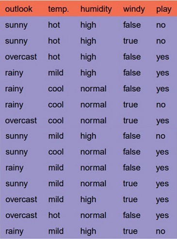
Let’s just take a famous dataset in the machine learning world which is weather dataset(playing game Y or N based on weather condition).
We have four X values (outlook,temp,humidity and windy) being categorical and one y value (play Y or N) also being categorical.
so we need to learn the mapping (what machine learning always does) between X and y.
This is a binary classification problem, lets build the tree using the ID3 algorithm
To create a tree, we need to have a root node first and we know that nodes are features/attributes(outlook,temp,humidity and windy),
Answer: determine the attribute that best classifies the training data; use this attribute at the root of the tree. Repeat this process at for each branch.
This means we are performing top-down, greedy search through the space of possible decision trees.
okayso how do we choose the best attribute?
Answer: use the attribute with the highest information gain in ID3 In order to define information gain precisely, we begin by defining a measure commonly used in information theory, called entropy that characterizes the (im)purity of an arbitrary collection of examples.”
For a binary classification problem
If all examples are positive or all are negative then entropy will be zero i.e, low.
If half of the examples are of positive class and half are of negative class then entropy is one i.e, high.
Okay lets apply these metrics to our dataset to split the data(getting the root node)
Steps:
1.compute the entropy for data-set2.for every attribute/feature:
       1.calculate entropy for all categorical values
       2.take average information entropy for the current attribute
       3.calculate gain for the current attribute3. pick the highest gain attribute.
4. Repeat until we get the tree we desired.
What the heck???
Okay I got it , if it does not make sense to you , let me make it sense to you. Compute the entropy for the weather data set:
For every feature calculate the entropy and information gain
Similary we can calculate for other two attributes(Humidity and Temp).
Pick the highest gain attribute.
So our root node isOutlook.
Repeat the same thing for sub-trees till we get the tree.
Classification with using the CART Algorithm:
In CART we use Gini index as a metric,
We use the Gini Index as our cost function used to evaluate splits in the dataset.
our target variable is Binary variable which means it take two values (Yes and No). There can be 4 combinations.
A Gini score gives an idea of how good a split is by how mixed the classes are in the two groups created by the split. A perfect separation results in a Gini score of 0, whereas the worst case split that results in 50/50 classes.
We calculate it for every row and split the data accordingly in our binary tree. We repeat this process recursively.
For Binary Target variable, Max Gini Index value
= 1 — (1/2)^2 — (1/2)^2
= 1–2*(1/2)^2 = 1- 2*(1/4) = 1–0.5 = 0.5
Similarly if Target Variable is categorical variable with multiple levels, the Gini Index will be still similar. If Target variable takes k different values, the Gini Index will be
Maximum value of Gini Index could be when all target values are equally distributed. Similarly for Nominal variable with k level, the maximum value Gini Index is = 1–1/k Minimum value of Gini Index will be 0 when all observations belong to one label.
Steps:
1.compute the gini index for data-set2.for every attribute/feature:
       1.calculate gini index for all categorical values
       2.take average information entropy for the current attribute
       3.calculate the gini gain3. pick the best gini gain attribute.
4. Repeat until we get the tree we desired.
The calculations are similar to ID3 ,except the formula changes.
for example :compute gini index for dataset
similarly we can follow other steps to build the trees.
Final Tree With All the Formulas.
Code For Decision Tree:
Note in the below snippet I have assumed that you have stored the dataset in the variable named df.
That’s it for this story. hope you enjoyed and learned something.