ML | Decision Tree Algorithm & Code using Python.

ML | Decision Tree Algorithm & Code using Python.

Decision Tree

Decision tree is one of the most popular machine learning algorithms used all along, This story I wanna talk about it so let’s get started!!!

Decision trees are used for both classification and regression problems, this story we talk about classification.

Before we dive into it , let me ask you this

Why Decision Tree?

We have couple of other algorithms there, so why do we have to choose Decision trees??

well, there might be many reasons but I believe a few which are

1. Decision tress often mimic the human level thinking so its so simple to understand the data and make some good interpretations.

1. Decision trees actually make you see the logic for the data to interpret(not like black box algorithms like SVM, NN, etc..)

For example : if we are classifying bank loan application for a customer, the decision tree may look like this

Here we can see the logic how it is making the decision.

It’s simple and clear.

 So what is the decision tree??

A decision tree is a tree where each node represents a feature(attribute), each link(branch) represents a decision(rule) and each leaf represents an outcome(categorical or continues value).

The whole idea is to create a tree like this for the entire data and process a single outcome at every leaf(or minimize the error in every leaf). 

Okay so how to build this??

There are couple of algorithms there to build a decision tree , we only talk about a few which are

1. CART (Classification and Regression Trees) → uses Gini Index(Classification) as metric.

1. ID3 (Iterative Dichotomiser 3) → uses Entropy function and Information gain as metrics.

Lets just first build decision tree for classification problem using above algorithms,

Classification with using the ID3 Algorithm.

Let’s just take a famous dataset in the machine learning world which is weather dataset(playing game Y or N based on weather condition).

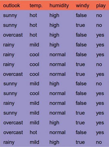
We have four X values (outlook,temp,humidity and windy) being categorical and one y value (play Y or N) also being categorical.

so we need to learn the mapping (what machine learning always does) between X and y.

This is a binary classification problem, lets build the tree using the ID3 algorithm

To create a tree, we need to have a root node first and we know that nodes are features/attributes(outlook,temp,humidity and windy),

Answer: determine the attribute that best classifies the training data; use this attribute at the root of the tree. Repeat this process at for each branch.

This means we are performing top-down, greedy search through the space of possible decision trees.

okay so how do we choose the best attribute?                        

 Answer: use the attribute with the highest information gain in ID3

In order to define information gain precisely, we begin by defining a measure commonly used in information theory, called entropy that characterizes the (im)purity of an arbitrary collection of examples.”

For a binary classification problem

• If all examples are positive or all are negative then entropy will be zero i.e, low.

• If half of the examples are of positive class and half are of negative class then entropy is one i.e, high.

Okay lets apply these metrics to our dataset to split the data(getting the root node)

Steps:

1.compute the entropy for data-set2.for every attribute/feature:
       1.calculate entropy for all categorical values
       2.take average information entropy for the current attribute
       3.calculate gain for the current attribute3. pick the highest gain attribute.
4. Repeat until we get the tree we desired.

What the heck???

Okay I got it , if it does not make sense to you , let me make it sense to you.

Compute the entropy for the weather data set:

For every feature calculate the entropy and information gain

 Similary we can calculate for other two attributes(Humidity and Temp).

Pick the highest gain attribute.

So our root node is Outlook.

Repeat the same thing for sub-trees till we get the tree.

Classification with using the CART Algorithm:

In CART we use Gini index as a metric,

We use the Gini Index as our cost function used to evaluate splits in the dataset.

our target variable is Binary variable which means it take two values (Yes and No). There can be 4 combinations.

Actual=1 predicted 1
1 0 , 0,1, 0 0P(Target=1).P(Target=1) + P(Target=1).P(Target=0) + P(Target=0).P(Target=1) + P(Target=0).P(Target=0) = 1P(Target=1).P(Target=0) + P(Target=0).P(Target=1) = 1 — P^2(Target=0) — P^2(Target=1)

Gini Index for Binary Target variable is

= 1 — P^2(Target=0) — P^2(Target=1)

Gini index

A Gini score gives an idea of how good a split is by how mixed the classes are in the two groups created by the split. A perfect separation results in a Gini score of 0, whereas the worst case split that results in 50/50 classes.

We calculate it for every row and split the data accordingly in our binary tree. We repeat this process recursively.

For Binary Target variable, Max Gini Index value

= 1 — (1/2)^2 — (1/2)^2

= 1–2*(1/2)^2
= 1- 2*(1/4)
= 1–0.5
= 0.5

Similarly if Target Variable is categorical variable with multiple levels, the Gini Index will be still similar. If Target variable takes k different values, the Gini Index will be

Maximum value of Gini Index could be when all target values are equally distributed.
Similarly for Nominal variable with k level, the maximum value Gini Index is
= 1–1/k
Minimum value of Gini Index will be 0 when all observations belong to one label.

Steps:

1.compute the gini index for data-set2.for every attribute/feature:
       1.calculate gini index for all categorical values
       2.take average information entropy for the current attribute 
       3.calculate the gini gain3. pick the best gini gain attribute.
4. Repeat until we get the tree we desired.

The calculations are similar to ID3 ,except the formula changes.

for example :compute gini index for dataset

similarly we can follow other steps to build the trees.

Final Tree With All the Formulas.

Code For Decision Tree:

Note in the below snippet I have assumed that you have stored the dataset in the variable named df.

That’s it for this story. hope you enjoyed and learned something.

Recommended Blogs:

1. How to become Data Scientist ? Skills required ? ( Click )

2. Machine Learning for beginners. ( Click )

3. ML | Linear Regression using Python ( Click )

Find me on Medium : Idrisi_Kasim

Thank You....: )

( Idrisi_Kasim )

ML | Linear Regression using Python.

ML | Linear Regression using Python.

Meaning of Regression

Regression attempts to predict one dependent variable (usually denoted by Y) and a series of other changing variables (known as independent variables, usually denoted by X).

Linear Regression

Linear Regression is a way of predicting a response Y on the basis of a single predictor variable X. It is assumed that there is approximately a linear relationship between X and Y. Mathematically, we can represent this relationship as:

Y ≈ ɒ + ß X + ℇ

where ɒ and ß are two unknown constants that represent intercept and slope terms in the linear model and ℇ is the error in the estimation.

Example

Let’s take the simplest possible example. Calculate the regression with only two data points.

Here we have 2 data points represented by two black points. All we are trying to do when we calculate our regression line is draw a line that is as close to every point as possible.

Here, we have a perfectly fitted line because we only have two points.Now, we have to consider a case where there are more than 2 data points.

By applying linear regression we can take multiple X’s and predict the corresponding Y values. This is depicted in the plot below:

Our goal with linear regression is to minimise the vertical distance between all the data points and our line.

So now I guess, you have got a basic idea what Linear Regression aims to achieve.

Before Applying any machine algorithm do Data Preparation Process to get the better results

Data Preparation Process

The more disciplined you are in your handling of data, the more consistent and better results you are like likely to achieve. The process for getting data ready for a machine learning algorithm can be summarized in three steps:

• Step 1: Select Data

• Step 2: Preprocess Data

• Step 3: Transform Data

You can follow this process in a linear manner, but it is very likely to be iterative with many loops.

Step 1: Select Data

This step is concerned with selecting the subset of all available data that you will be working with. There is always a strong desire for including all data that is available, that the maxim “more is better” will hold. This may or may not be true.

You need to consider what data you actually need to address the question or problem you are working on. Make some assumptions about the data you require and be careful to record those assumptions so that you can test them later if needed.

Below are some questions to help you think through this process:

• What is the extent of the data you have available? For example through time, database tables, connected systems. Ensure you have a clear picture of everything that you can use.

• What data is not available that you wish you had available? For example data that is not recorded or cannot be recorded. You may be able to derive or simulate this data.

• What data don’t you need to address the problem? Excluding data is almost always easier than including data. Note down which data you excluded and why.

It is only in small problems, like competition or toy datasets where the data has already been selected for you.

Step 2: Preprocess Data

After you have selected the data, you need to consider how you are going to use the data. This preprocessing step is about getting the selected data into a form that you can work.

Three common data preprocessing steps are formatting, cleaning and sampling:

• Formatting: The data you have selected may not be in a format that is suitable for you to work with. The data may be in a relational database and you would like it in a flat file, or the data may be in a proprietary file format and you would like it in a relational database or a text file.

• Cleaning: Cleaning data is the removal or fixing of missing data. There may be data instances that are incomplete and do not carry the data you believe you need to address the problem. These instances may need to be removed. Additionally, there may be sensitive information in some of the attributes and these attributes may need to be anonymized or removed from the data entirely.

• Sampling: There may be far more selected data available than you need to work with. More data can result in much longer running times for algorithms and larger computational and memory requirements. You can take a smaller representative sample of the selected data that may be much faster for exploring and prototyping solutions before considering the whole dataset.

It is very likely that the machine learning tools you use on the data will influence the preprocessing you will be required to perform. You will likely revisit this step.

Step 3: Transform Data

The final step is to transform the process data. The specific algorithm you are working with and the knowledge of the problem domain will influence this step and you will very likely have to revisit different transformations of your preprocessed data as you work on your problem.

Three common data transformations are scaling, attribute decompositions and attribute aggregations. This step is also referred to as feature engineering.

• Scaling: The preprocessed data may contain attributes with a mixtures of scales for various quantities such as dollars, kilograms and sales volume. Many machine learning methods like data attributes to have the same scale such as between 0 and 1 for the smallest and largest value for a given feature. Consider any feature scaling you may need to perform.

• Decomposition: There may be features that represent a complex concept that may be more useful to a machine learning method when split into the constituent parts. An example is a date that may have day and time components that in turn could be split out further. Perhaps only the hour of day is relevant to the problem being solved. consider what feature decompositions you can perform.

• Aggregation: There may be features that can be aggregated into a single feature that would be more meaningful to the problem you are trying to solve. For example, there may be a data instances for each time a customer logged into a system that could be aggregated into a count for the number of logins allowing the additional instances to be discarded. Consider what type of feature aggregations could perform.

You can spend a lot of time engineering features from your data and it can be very beneficial to the performance of an algorithm. Start small and build on the skills you learn.

Steps for Linear Regression:  

1. Importing the necessary Libraries & dataset.

2. Splitting the dataset into the Training set and Test set.

3. Fitting Simple Linear Regression to the Training set.

4. Predicting the Test set results.

5. Scatter plot of y_test vs Prediction.

6. Distplot...( Should come Normal distribution otherwise eliminate Linear Reg )

7. Visualizing the Training set results ( Optional )

8. Visualizing the Test set results ( Optional )

9. Lets Predict...!

10. Also Calculate: coef_ , intercept_ , MAE , MSE , RMSE , r2_score.

Code for Linear Regression:

In the below code snippet I have assumed the dataset is stored in the variable df.

To find Accuracy, Mean Absolute Error, Mean Squared Error, Root Mean Squared error execute the following code.

Please also import this in below code since i have forget to mention sklearn.metrics import r2_score.

Mathematical Formula for all the above error

Recommended Blogs:

1. How to become Data Scientist ? Skills required ? ( Click )

2. Machine Learning for beginners. ( Click )

3. ML | LogisticRegression Algorithm ( Click )

4. ML | Decision Tree Algorithm & Code using Python. ( Click )

5. ML | RandomForest Algorithm. ( Click )

Find me on Medium : Idrisi_Kasim

Find me on Github : Kasim8630

Thank You....: )

( Idrisi_Kasim )